
Microeconomic Review
- Resevation price: a person's maximum willingness to pay for sth
- Utility is simply a way of describing preferences.
- A Utility Function is a way of assigning a number to every possible consumption bundle such that more-preferred bundles get assigned larger numbers than less-preferred bundles
- Ordinal Utility: The magnitude of the utility function is only important to rank the different consumption bundles; the size of the utility difference between any two consumption bundles doesn't matter.
- Monotonic Transformation is a way of transforming one set of numbers into another set of numbers in a way that preserves the order of the numbers.
- a monotonic transformation of a utility function is a utility function that represents the same preferences as the original utility function.
- Cardinal Utility: attach a significance to the magnitude of utility.
- A utility function is simply a way to represent or summarize a preference ordering. The numerical magnitudes of utility levels have no intrinsic meaning.
- \(MRS = -\frac{MU_1}{MU_2}\)
Optimal Choice: the indifference curve is tangent to the budget line.
Demand Functions give the optimal amounts of each of the goods as a function of the prices and income faced by the consumer
Normal Goods: the demand for it increases when income increases.
Inferior Good: the demand for it decreases when income increases.
Engel curve is a graph of the demand for one of the goods as a function of income, with all prices being held constant.
an increase in income corresponds to shifting the budget line outward in a parallel manner. We can connect together the demanded bundles that we get as we shift the budget line outward to construct the income offer curve.
Ordinary Good: the demand for a good increases when its price decreases.
Giffen Good: the demand for it decreases when its price decreases.
Suppose that we let the price of good 1 change while we hold \[p_2\] and income fixed. Geometrically this involves pivoting the budget line. We can connect together the optimal points to construct the price offer curve.
Demand Curve: hold the price of good 2 and money income fixed, and for each different value of \(p_1\) plot the optimal level of consumption of good 1.
If the demand for good 1 increases when the price of good 2 increases, then good 1 is a substitute for good 2. If the demand for good 1 decreases in this situation, then it is a complement for good 2.
When the price of a good changes, there are two sorts of effects: the rate at which you can exchange one good for another changes(substitution effect), and the total purchasing power of your income is altered(income effect).
This “pivot-shift” operation gives us a convenient way to decompose the change in demand into two pieces. The first step—the pivot—is a movement where the slope of the budget line changes while its purchasing power stays constant, while the second step is a movement where the slope stays constant and the purchasing power changes
the substitution effect must always be negative—opposite the change in the price—the income effect can go either way. Thus the total effect may be positive or negative.
Thus a Giffen good must be an inferior good. But an inferior good is not necessarily a Giffen good
The Law of Demand: If the demand for a good increases when income increases, then the demand for that good must decrease when its price increases.
Hicks substitution effect: Suppose that instead of pivoting the budget line around the original consumption bundle, we now roll the budget line around the indifference curve through the original consumption bundle
Thus the Hicks substitution effect keeps utility constant rather than keeping purchasing power constant.
When the price of a good decreases, there will be two effects on consumption. The change in relative prices makes the consumer want to consume more of the cheaper good. The increase in purchasing power due to the lower price may increase or decrease consumption, depending on whether the good is a normal good or an inferior good.
The change in demand due to the change in relative prices is called the substitution effect; the change due to the change in purchasing power is called the income effect.
Economics is the study of how society manages its scarce resources
Scarcity the limited nature of society’s resources
The opportunity cost of an item is what you give up to get that item
A market is a group of buyers and sellers of a particular good or service.
Economists use the term competitive market to describe a market in which there are so many buyers and so many sellers that each has a negligible impact on the market price.
Perfectly Competitive: To reach this highest form of competition, a market must have two characteristics: (1) The goods offered for sale are all exactly the same, and (2) the buyers and sellers are so numerous that no single buyer or seller has any influence over the market price.
Because buyers and sellers in perfectly competitive markets must accept the price the market determines, they are said to be price takers.
Some markets have only one seller, and this seller sets the price. Such a seller is called a monopoly.
The quantity demanded of any good is the amount of the good that buyers are willing and able to purchase.
The line relating price and quantity demanded is called the demand curve
market demand, the sum of all the individual demands for a particular good or service. Thus, the market demand curve is found by adding horizontally the individual demand curves.
Any change that raises the quantity that buyers wish to purchase at any given price shifts the demand curve to the right. Any change that lowers the quantity that buyers wish to purchase at any given price shifts the demand curve to the left.
a change in the good’s price represents a movement along the demand curve, whereas a change in one of the other variables shifts the demand curve.
The quantity supplied of any good or service is the amount that sellers are willing and able to sell.
The curve relating price and quantity supplied is called the supply curve
a change in the good’s price represents a movement along the supply curve, whereas a change in one of the other variables shifts the supply curve.
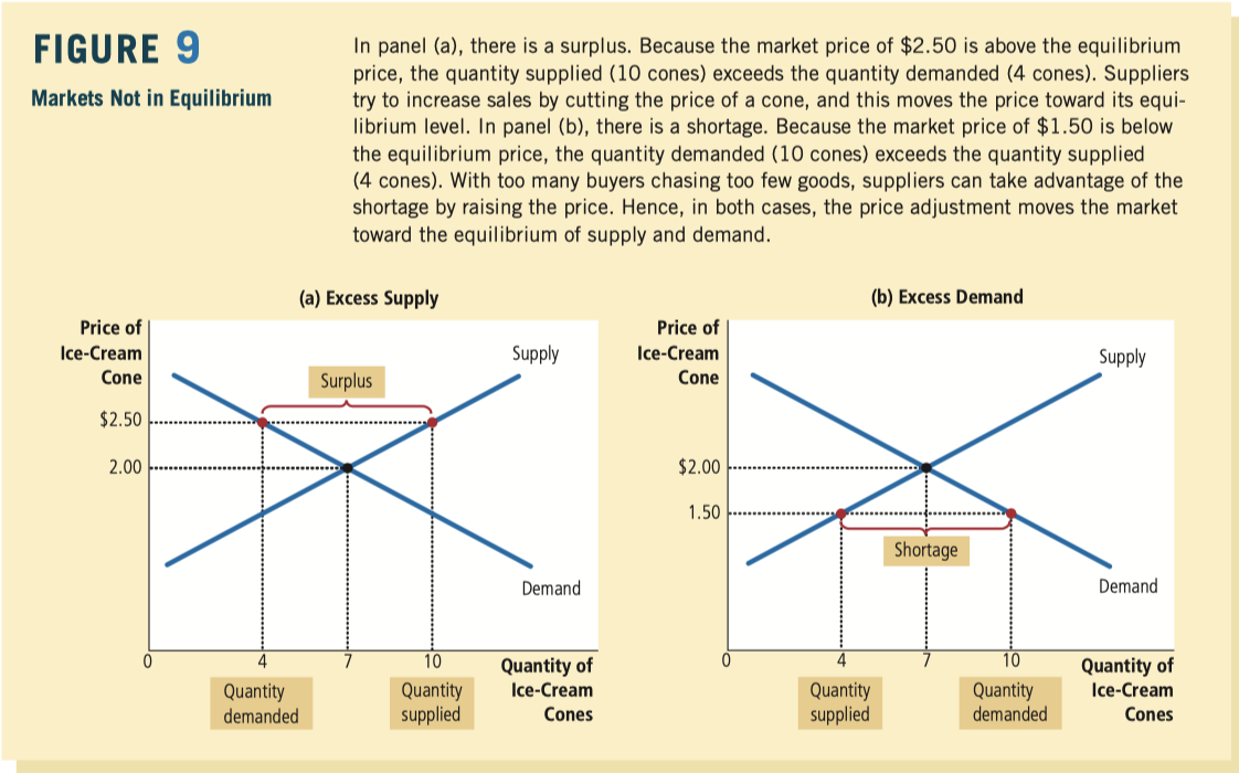
Notice that there is one point at which the supply and demand curves intersect. This point is called the market’s equilibrium. The price at this intersection is called the equilibrium price, and the quantity is called the equilibrium quantity
At the equilibrium price, the quantity of the good that buyers are willing and able to buy exactly balances the quantity that sellers are willing and able to sell. The equilibrium price is sometimes called the market-clearing price because, at this price, everyone in the market has been satisfied: Buyers have bought all they want to buy, and sellers have sold all they want to sell
![image-20200101201023877]()
a shift in the supply curve is called a “change in supply,” and a shift in the demand curve is called a “change in demand.” A movement along a fixed supply curve is called a “change in the quantity supplied,” and a movement along a fixed demand curve is called a “change in the quantity demanded.”
The price elasticity of demand measures how much the quantity demanded responds to a change in price. Demand for a good is said to be elastic if the quantity demanded responds substantially to changes in the price. Demand is said to be inelastic if the quantity demanded responds only slightly to changes in the price.
Necessities versus Luxuries Necessities tend to have inelastic demands, whereas luxuries have elastic demands
Total revenue
- When demand is inelastic (a price elasticity less than 1), price and total revenue move in the same direction: If the price increases, total revenue also increases.
- When demand is elastic (a price elasticity greater than 1), price and total revenue move in opposite directions: If the price increases, total revenue decreases.
- If demand is unit elastic (a price elasticity exactly equal to 1), total revenue remains constant when the price changes.
The income elasticity of demand measures how the quantity demanded changes as consumer income changes
- Most goods are normal goods: Higher income raises the quantity demanded. Because quantity demanded and income move in the same direction, normal goods have positive income elasticities.
- A few goods, such as bus rides, are inferior goods: Higher income lowers the quantity demanded. Because quantity demanded and income move in opposite directions, inferior goods have negative income elasticities.
- Necessities, such as food and clothing, tend to have small income elasticities because consumers choose to buy some of these goods even when their incomes are low.
- Luxuries, such as caviar and diamonds, tend to have large income elasticities because consumers feel that they can do without these goods altogether if their incomes are too low.
The cross-price elasticity of demand measures how the quantity demanded of one good responds to a change in the price of another good.
- Substitute : positive
- Complement : negative
The price elasticity of supply measures how much the quantity supplied responds to changes in the price.
![image-20200102141337326]()
Because the price is not allowed to rise above this level, the legislated maximum is called a price ceiling
Because the price cannot fall below this level, the legislated minimum is called a price floor.
When the government imposes a binding price ceiling on a competitive market, a shortage of the good arises, and sellers must ration the scarce goods among the large number of potential buyers.
![image-20200102203156995]()
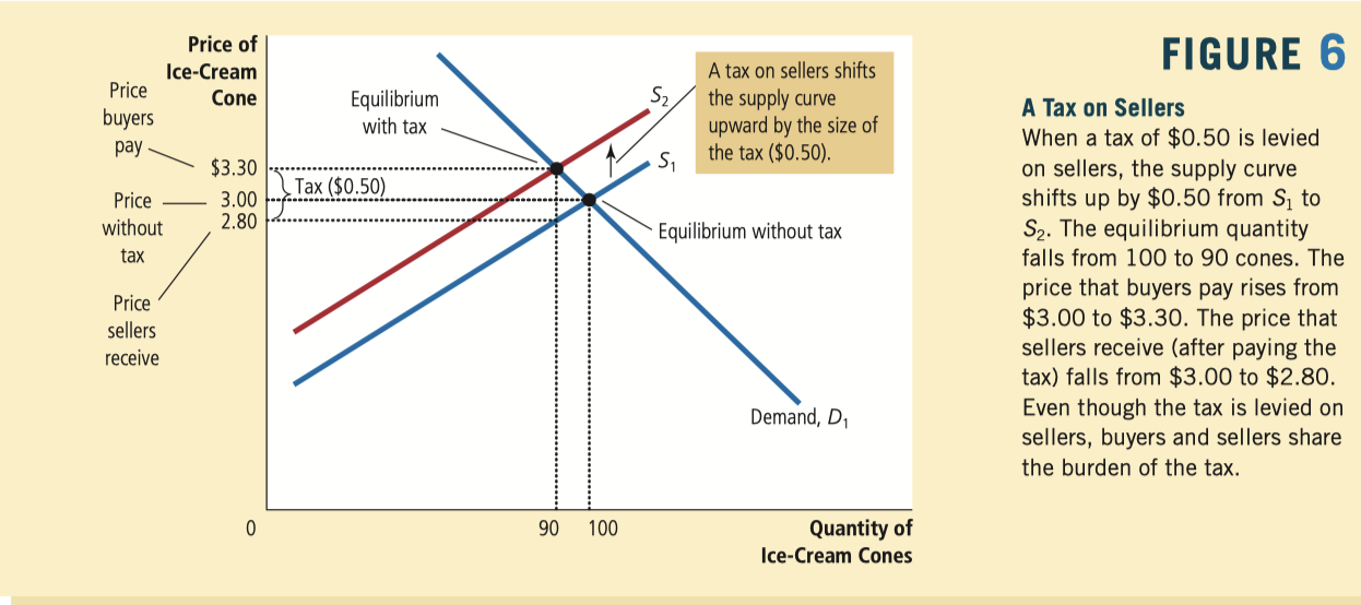
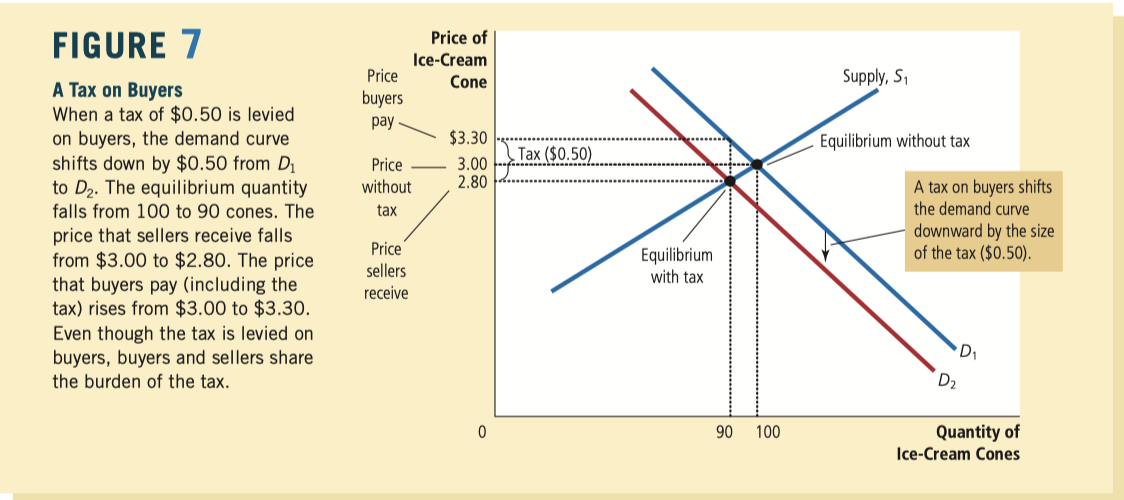
- Taxes discourage market activity. When a good is taxed, the quantity of the good sold is smaller in the new equilibrium.
- Buyers and sellers share the burden of taxes. In the new equilibrium, buyers pay more for the good, and sellers receive less.
![image-20200102212038172]()
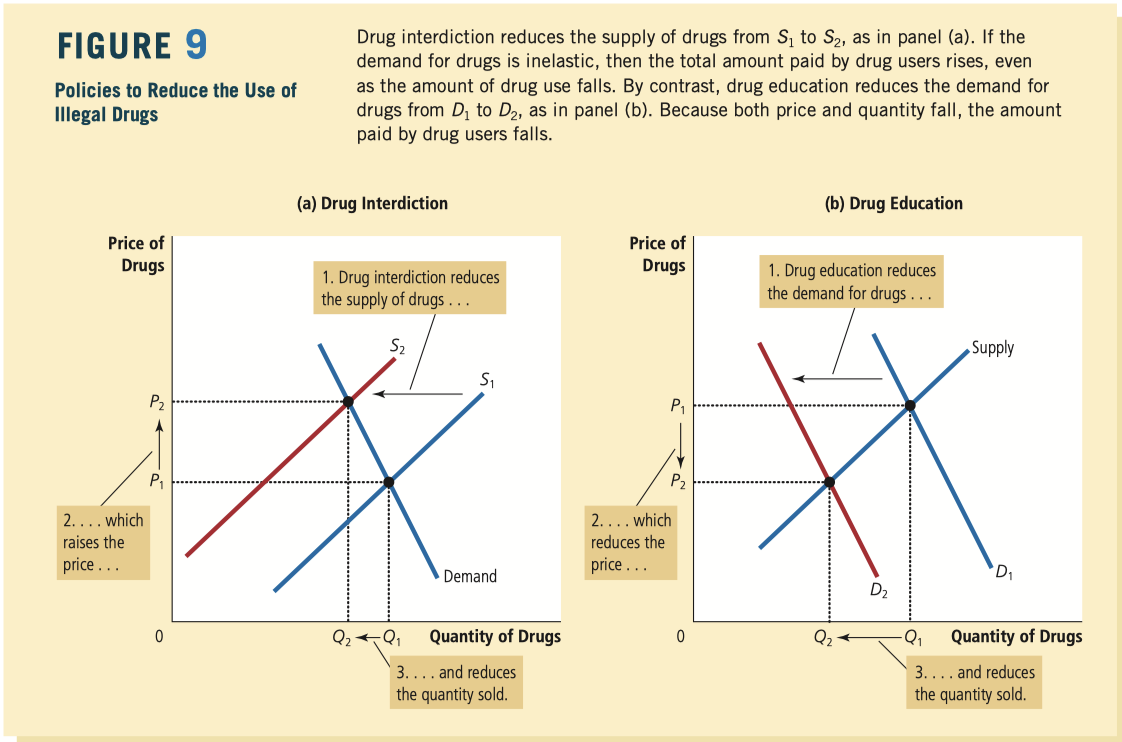
The incidence of a tax depends on the price elasticities of supply and demand. Most of the burden falls on the side of the market that is less elastic because that side of the market cannot respond as easily to the tax by changing the quantity bought or sold.
welfare economics the study of how the allocation of resources affects economic well-being
willingness to pay: the maximum amount that a buyer will pay for a good
Consumer surplus is the amount a buyer is willing to pay for a good minus the amount the buyer actually pays for it. Consumer surplus measures the benefit buyers receive from participating in a market.
The area below the demand curve and above the price measures the consumer surplus in a market.
Producer surplus is the amount a seller is paid minus the cost of production. Producer surplus measures the benefit sellers receive from participating in a market.
The area below the price and above the supply curve measures the producer surplus in a market.
externalities: buyers and sellers may ignore some side effects when deciding how much to consume and produce, the equilibrium in a market can be inefficient from the standpoint of society as a whole.
market failure—the inability of some unregulated markets to allocate resources efficiently.
deadweight loss: the fall in total surplus that results from a market distortion, such as a tax
Taxes cause deadweight losses because they prevent buyers and sellers from realizing some of the gains from trade.
the greater the elasticities of supply and demand, the greater the deadweight loss of a tax.
![image-20200103132936210]()
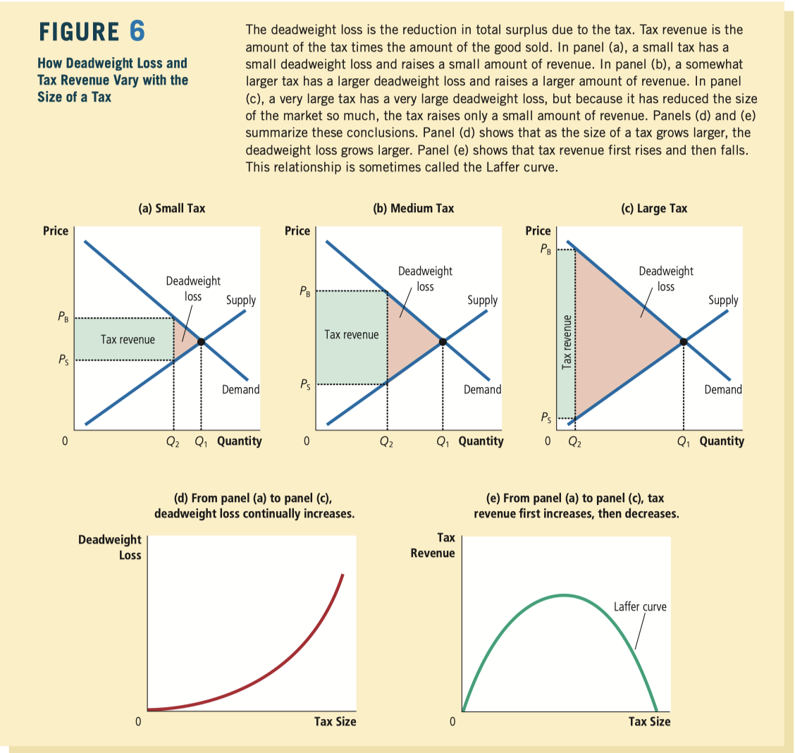
A tax on a good reduces the welfare of buyers and sellers of the good, and the reduction in consumer and producer surplus usually exceeds the revenue raised by the government. The fall in total surplus—the sum of consumer surplus, producer surplus, and tax revenue—is called the deadweight loss of the tax.
Taxes have deadweight losses because they cause buyers to consume less and sellers to produce less, and these changes in behavior shrink the size of the market below the level that maximizes total surplus. Because the elasticities of supply and demand measure how much market participants respond to market conditions, larger elasticities imply larger deadweight losses.
As a tax grows larger, it distorts incentives more, and its deadweight loss grows larger. Because a tax reduces the size of the market, however, tax revenue does not continually increase. It first rises with the size of a tax, but if the tax gets large enough, tax revenue starts to fall.
An externality arises when a person engages in an activity that influences the well-being of a bystander but neither pays nor receives compensation for that effect.
- If the impact on the bystander is adverse, it is called a negative externality.
- If it is beneficial, it is called a positive externality
internalizing the externality altering incentives so that people take account of the external effects of their actions
Negative externalities lead markets to produce a larger quantity than is socially desirable. Positive externalities lead markets to produce a smaller quantity than is socially desirable. To remedy the problem, the government can internalize the externality by taxing goods that have negative externalities and subsidizing goods that have positive externalities.
Coase theorem: the proposition that if private parties can bargain without cost over the allocation of resources, they can solve the problem of externalities on their own
The Coase theorem says that private economic actors can potentially solve the problem of externalities among themselves. Whatever the initial distribution of rights, the interested parties can reach a bargain in which everyone is better off and the outcome is efficient.
Governments pursue various policies to remedy the inefficiencies caused by externalities. Sometimes the government prevents socially inefficient activity by regulating behavior. Other times it internalizes an externality using corrective taxes. Another public policy is to issue permits. For example, the government could protect the environment by issuing a limited number of pollution permits. The result of this policy is largely the same as imposing corrective taxes on polluters.
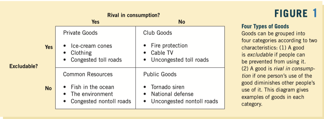
Excludability the property of a good whereby a person can be prevented from using it
Rivalry in consumption the property of a good whereby one person’s use diminishes other people’s use
Private goods are both excludable and rival in consumption.
Public goods are neither excludable nor rival in consumption.
Common resources are rival in consumption but not excludable
Club goods are excludable but not rival in consumption
![image-20200103144802240]()
free rider a person who receives the benefit of a good but avoids paying for it
Because public goods are not excludable, the free-rider problem prevents the private market from supplying them. The government, however, can potentially remedy the problem. If the government decides that the total benefits of a public good exceed its costs, it can provide the public good, pay for it with tax revenue, and make everyone better off.
Public goods are neither rival in consumption nor excludable. Examples of public goods include fireworks displays, national defense, and the creation of fundamental knowledge. Because people are not charged for their use of the public good, they have an incentive to free ride, making private provision of the good untenable. Therefore, governments provide public goods, basing their decision about the quantity of each good on cost–benefit analysis.
Common resources are rival in consumption but not excludable. Examples include common grazing land, clean air, and congested roads. Because people are not charged for their use of common resources, they tend to use them excessively. Therefore, governments use various methods to limit the use of common resources.
Total Revenue the amount a firm receives for the sale of its output
Total Cost the market value of the inputs a firm uses in production
Profit total revenue minus total cost
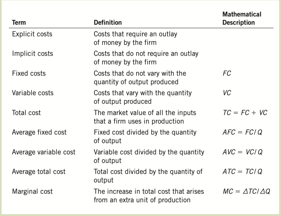
Explicit Costs input costs that require an outlay of money by the firm
Implicit Costs input costs that do not require an outlay of money by the firm
Economic Profit total revenue minus total cost, including both explicit and implicit costs
Accounting Profit total revenue minus total explicit cost
Production Function the relationship between quantity of inputs used to make a good and the quantity of output of that good
Marginal Product the increase in output that arises from an additional unit of input
Diminishing Marginal Product the property whereby the marginal product of an input declines as the quantity of the input increases
Fixed Costs costs that do not vary with the quantity of output produced
Variable Costs costs that vary with the quantity of output produced
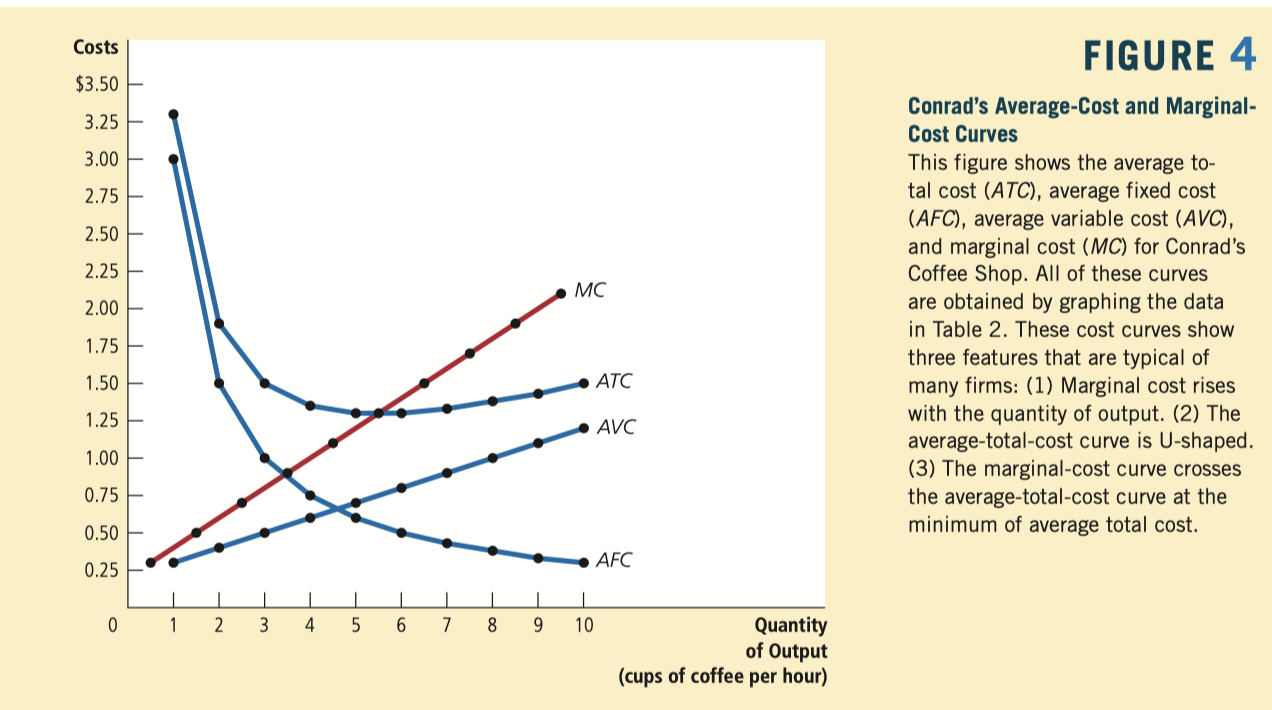
Average Total Cost total cost divided by the quantity of output
Average Fixed Cost fixed cost divided by the quantity of output
Average Variable Cost variable cost divided by the quantity of output
Marginal Cost the increase in total cost that arises from an extra unit of production
![image-20200103153735311]()
Efficient Scale the quantity of output that minimizes average total cost
Whenever marginal cost is less than average total cost, average total cost is falling. Whenever marginal cost is greater than average total cost, average total cost is rising.
The marginal-cost curve crosses the average-total-cost curve at its minimum.
![image-20200103154827862]()
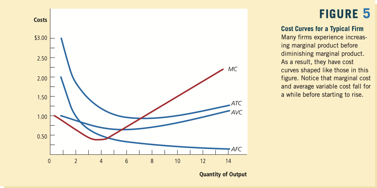
- Marginal cost eventually rises with the quantity of output.
- The average-total-cost curve is U-shaped.
- The marginal-cost curve crosses the average-total-cost curve at the minimum of average total cost.
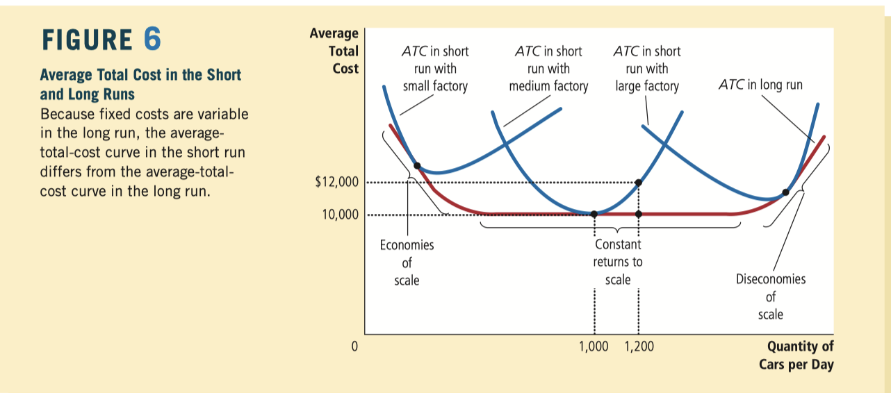
![image-20200103155338794]()
- Economies Of Scale the property whereby long-run average total cost falls as the quantity of output increases
- Diseconomies Of Scale the property whereby long-run average total cost rises as the quantity of output increases
- Constant Returns to scale the property whereby long-run average total cost stays the same as the quantity of output changes
![image-20200103155618866]()
Competitive Market a market with many buyers and sellers trading identical products so that each buyer and seller is a price taker.
- There are many buyers and many sellers in the market.
- The goods offered by the various sellers are largely the same.
- Firms can freely enter or exit the market.
For all types of firms, average revenue equals the price of the good.
For competitive firms, marginal revenue equals the price of the good.
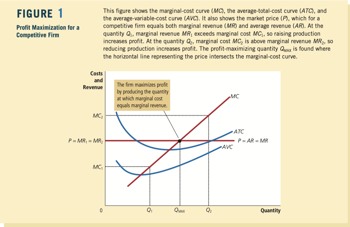
![image-20200103161648108]()
- If marginal revenue is greater than marginal cost, the firm should increase its output.
- If marginal cost is greater than marginal revenue, the firm should decrease its output.
- At the profit-maximizing level of output, marginal revenue and marginal cost are exactly equal.
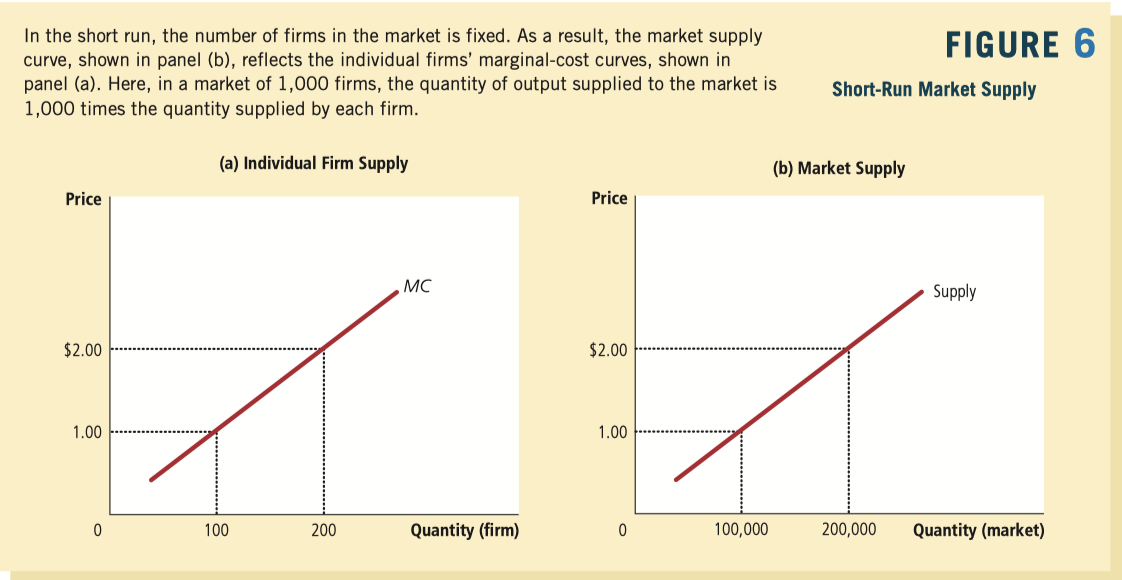
In essence, because the firm’s marginal-cost curve determines the quantity of the good the firm is willing to supply at any price, the marginal-cost curve is also the competitive firm’s supply curve.
A shutdown refers to a short-run decision not to produce anything during a specific period of time because of current market conditions. Exit refers to a long-run decision to leave the market. The short-run and long-run decisions differ because most firms cannot avoid their fixed costs in the short run but can do so in the long run. That is, a firm that shuts down temporarily still has to pay its fixed costs, whereas a firm that exits the market does not have to pay any costs at all, fixed or variable.
The competitive firm’s short-run supply curve is the portion of its marginal-cost curve that lies above average variable cost.
The competitive firm’s long-run supply curve is the portion of its marginal-cost curve that lies above average total cost.
the firm shuts down if the revenue that it would earn from producing is less than its variable costs of production.
sunk cost a cost that has already been committed and cannot be recovered
![image-20200103162830530]()
![image-20200103162818679]()
Economic Profit is zero, but Accounting Profit is positive
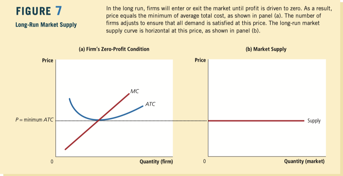
![image-20200103163407036]()
In the short run when a firm cannot recover its fixed costs, the firm will choose to shut down temporarily if the price of the good is less than average variable cost. In the long run when the firm can recover both fixed and variable costs, it will choose to exit if the price is less than average total cost.
In a market with free entry and exit, profit is driven to zero in the long run. In this long-run equilibrium, all firms produce at the efficient scale, price equals the minimum of average total cost, and the number of firms adjusts to satisfy the quantity demanded at this price.
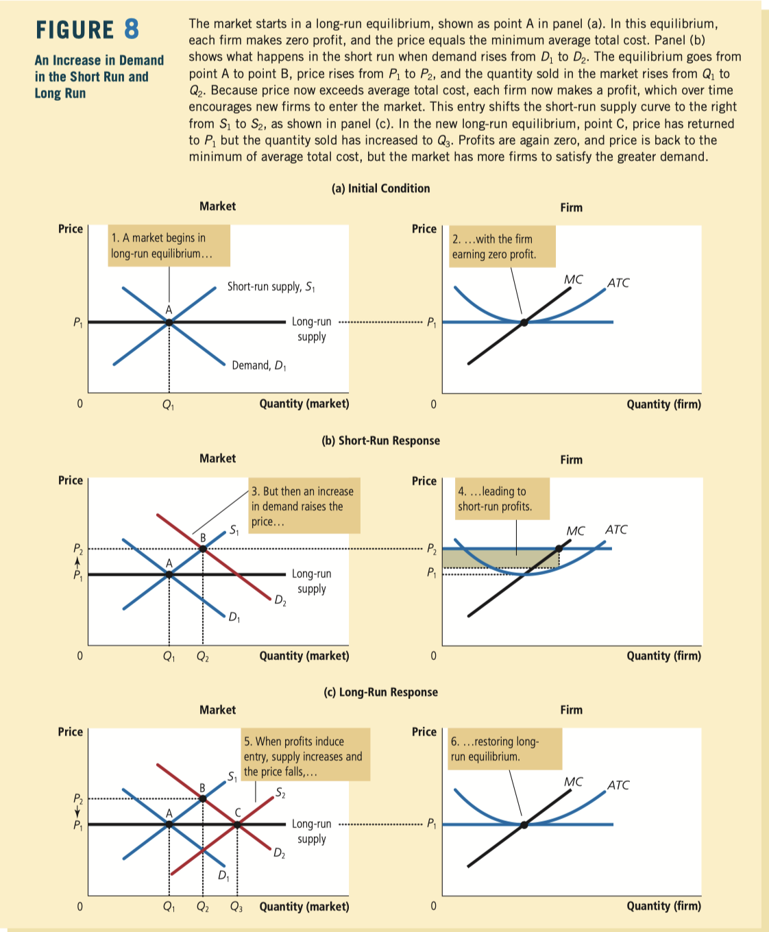
Changes in demand have different effects over different time horizons. In the short run, an increase in demand raises prices and leads to profits, and a decrease in demand lowers prices and leads to losses. But if firms can freely enter and exit the market, then in the long run, the number of firms adjusts to drive the market back to the zero-profit equilibrium.
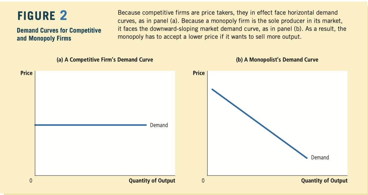
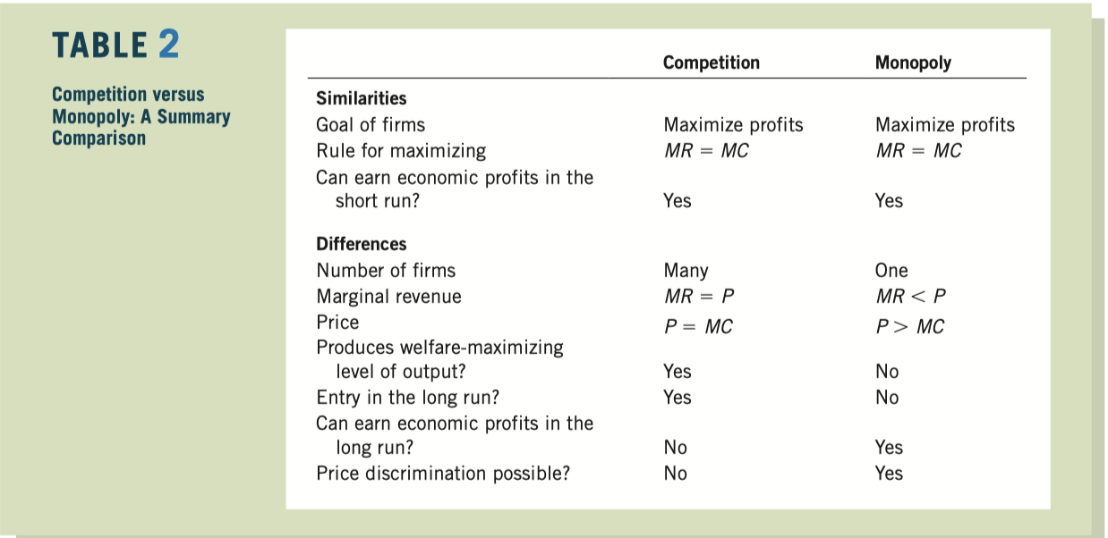
a competitive firm is a price taker, a monopoly firm is a price maker
Barriers to Entry: A monopoly remains the only seller in its market because other firms cannot enter the market and compete with it. Barriers to entry, in turn, have three main sources:
- Monopoly resources: A key resource required for production is owned by a single firm.
- Government regulation: The government gives a single firm the exclusive right to produce some good or service.
- The patent and copyright laws are two important examples
- The production process: A single firm can produce output at a lower cost than can a larger number of firms.
Natural Monopoly a monopoly that arises because a single firm can supply a good or service to an entire market at a smaller cost than could two or more firms
![image-20200103195210478]()
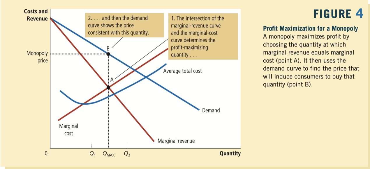
![image-20200103195434964]()
![image-20200103195538613]()
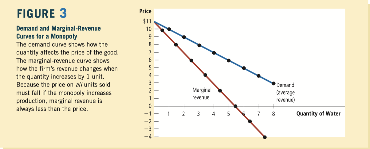
the monopolist’s profit-maximizing quantity of output is determined by the intersection of the marginalrevenue curve and the marginal-cost curve.
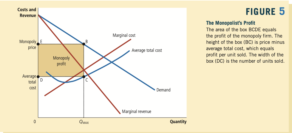
![image-20200103200013666]()
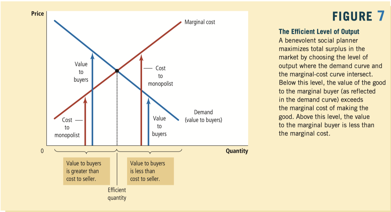
![image-20200103202115329]()
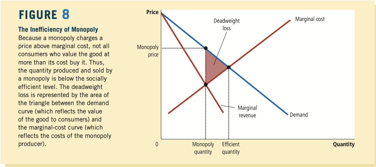
![image-20200103202342327]()
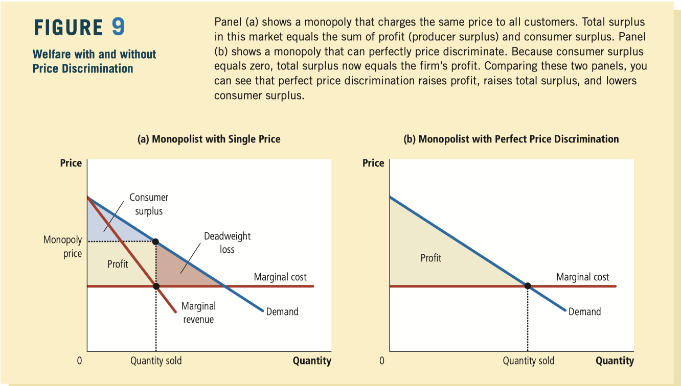
Price Discrimination the business practice of selling the same good at different prices to different customers
Perfect price discrimination describes a situation in which the monopolist knows exactly each customer’s willingness to pay and can charge each customer a different price.
![image-20200103204726504]()
monopolists price discriminate by charging different prices to the same customer for different units that the customer buys.
Public Policy toward Monopolies
- By trying to make monopolized industries more competitive.
- Increasing Competition with Antitrust Laws (cost:synergies)
- By regulating the behavior of the monopolies.
- By turning some private monopolies into public enterprises.
- Public Ownership
- By doing nothing at all.
- By trying to make monopolized industries more competitive.
![image-20200103211333718]()
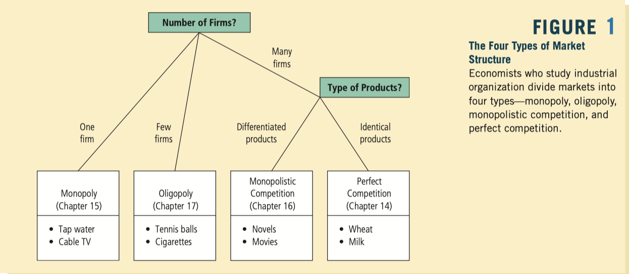
oligopoly a market structure in which only a few sellers offer similar or identical products
monopolistic competition a market structure in which many firms sell products that are similar but not identical
- Many sellers: There are many firms competing for the same group of customers.
- Product differentiation: Each firm produces a product that is at least slightly different from those of other firms. Thus, rather than being a price taker, each firm faces a downward-sloping demand curve.
- Free entry and exit: Firms can enter or exit the market without restriction. Thus, the number of firms in the market adjusts until economic profits are driven to zero.
![image-20200103213234782]()
![image-20200103215610700]()
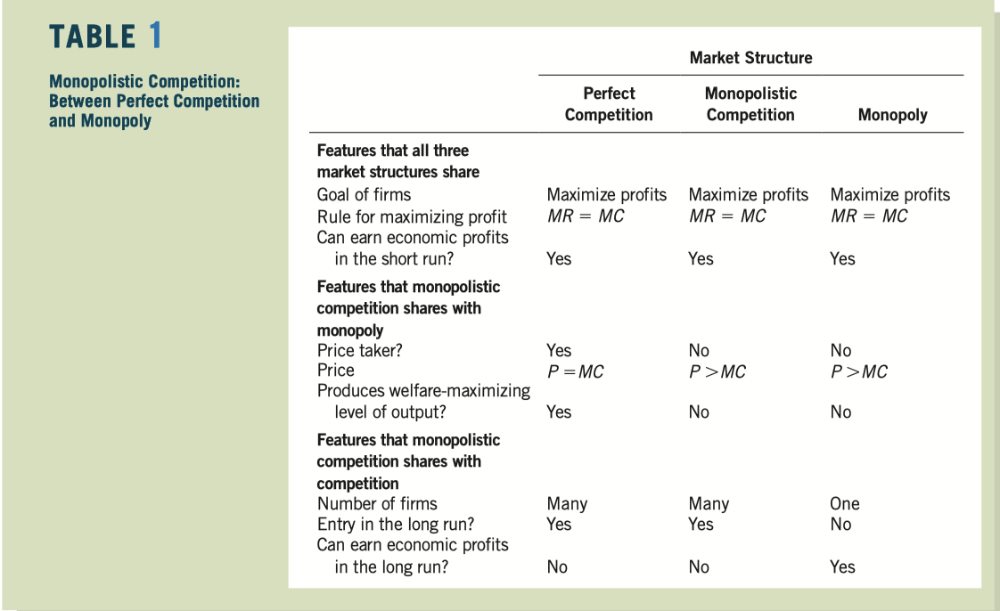
The long-run equilibrium in a monopolistically competitive market differs from that in a perfectly competitive market in two related ways.
- First, each firm in a monopolistically competitive market has excess capacity. That is, it chooses a quantity that puts it on the downward-sloping portion of the average-total-cost curve.
- Second, each firm charges a price above marginal cost.
Game Theory the study of how people behave in strategic situation
Collusion an agreement among firms in a market about quantities to produce or prices to charge
Cartel a group of firms acting in unison
Nash equilibrium a situation in which economic actors interacting with one another each choose their best strategy given the strategies that all the other actors have chosen
Oligopolists maximize their total profits by forming a cartel and acting like a monopolist. Yet, if oligopolists make decisions about production levels individually, the result is a greater quantity and a lower price than under the monopoly outcome. The larger the number of firms in the oligopoly, the closer the quantity and price will be to the levels that would prevail under perfect competition.
Capital the equipment and structures used to produce goods and services
In many economic transactions, information is asymmetric. When there are hidden actions, principals may be concerned that agents suffer from the problem of moral hazard. When there are hidden characteristics, buyers may be concerned about the problem of adverse selection among the sellers. Private markets sometimes deal with asymmetric information with signaling and screening.
If a good has an elasticity of demand greater than 1 in absolute value we say that it has an elastic demand. If the elasticity is less than 1 in absolute value we say that it has an inelastic demand. And if it has an elasticity of exactly −1, we say it has unit elastic demand.
If demand is very responsive to price—that is, it is very elastic—then an increase in price will reduce demand so much that revenue will fall. If demand is very unresponsive to price—it is very inelastic—then an increase in price will not change demand very much, and overall revenue will increase.
Constant Elasticity Demands: the logarithm of q depends in a linear way on the logarithm of p
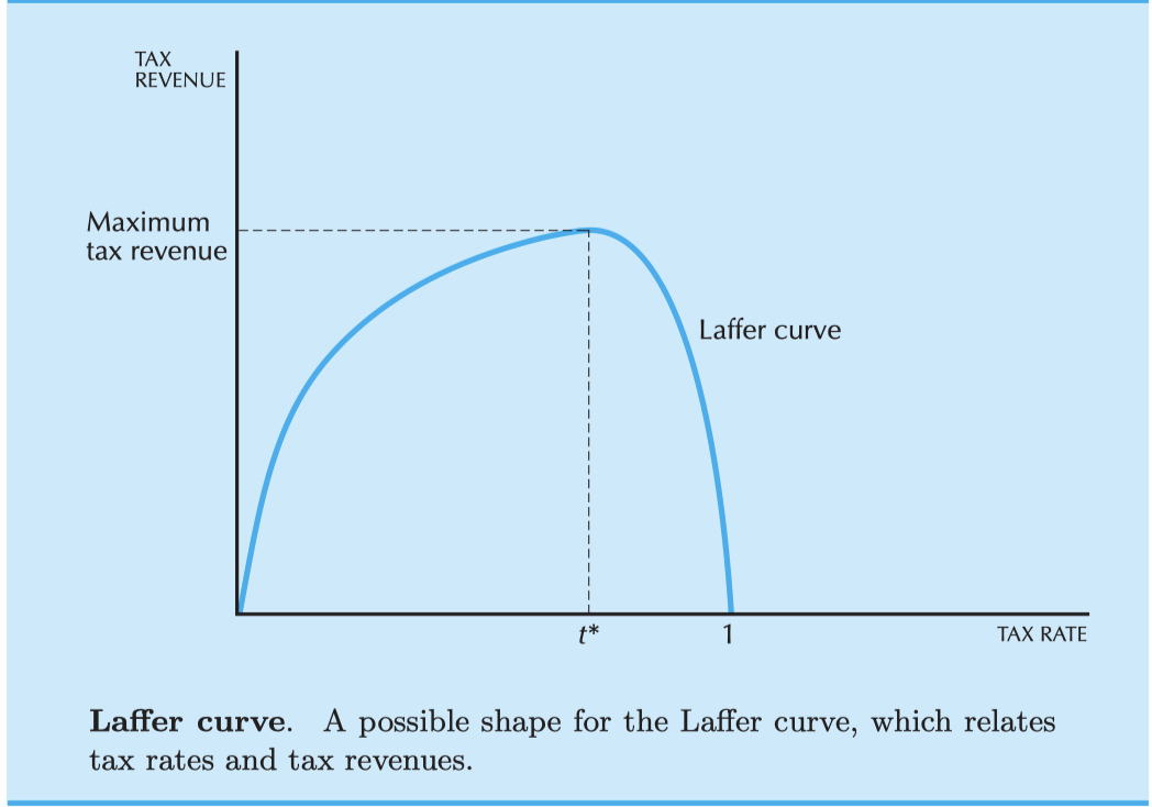
![image-20200108124537772]()
- The interesting feature of the Laffer curve is that it suggests that when the tax rate is high enough, an increase in the tax rate will end up reducing the revenues collected. The reduction in the supply of the good due to the increase in the tax rate can be so large that tax revenue actually decreases.
Pareto efficient if there is no way to make any person better off without hurting anybody else.
An equilibrium price is one where the quantity that people are willing to supply equals the quantity that people are willing to demand.
How much of a tax gets passed along to consumers depends on the relative steepness of the demand and supply curves. If the supply curve is horizontal, all of the tax gets passed along to consumers; if the supply curve is vertical, none of the tax gets passed along.
An isoquant (等产量线) is the set of all possible combinations of inputs 1 and 2 that are just sufficient to produce a given amount of output.
Returns to scale describes what happens when you increase all inputs, while diminishing marginal product describes what happens when you increase one of the inputs and hold the others fixed.
The technological constraints of the firm are described by the production set, which depicts all the technologically feasible combinations of inputs and outputs, and by the production function, which gives the maximum amount of output associated with a given amount of the inputs.
The technical rate of substitution (TRS) measures the slope of an isoquant.
Returns to scale refers to the way that output changes as we change the scale of production. If we scale all inputs up by some amount t and output goes up by the same factor, then we have constant returns to scale. If output scales up by more that t, we have increasing returns to scale; and if it scales up by less than t, we have decreasing returns to scale.
Fixed factors are factors whose amount is independent of the level of output; variable factors are factors whose amount used changes as the level of output changes.
If the firm is maximizing profits, then the value of the marginal product of each factor that it is free to vary must equal its factor price.
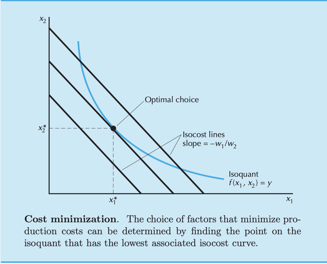
![image-20200108144329763]()
The short-run cost function is defined as the minimum cost to produce a given level of output, only adjusting the variable factors of production. The long-run cost function gives the minimum cost of producing a given level of output, adjusting all of the factors of production.
The average variable cost curve may initially slope down but need not. However, it will eventually rise, as long as there are fixed factors that constrain production.
The average cost curve will initially fall due to declining fixed costs but then rise due to the increasing average variable costs.
The marginal cost and average variable cost are the same at the first unit of output.
The marginal cost curve passes through the minimum point of both the average variable cost and the average cost curves.
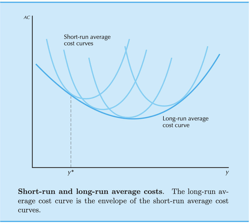
![image-20200108151228878]()
long-run average cost curve is the lower envelope (下包络线) of the short-run average cost curves.
Average costs are composed of average variable costs plus average fixed costs. Average fixed costs always decline with output, while average variable costs tend to increase. The net result is a U-shaped average cost curve.
The marginal cost curve lies below the average cost curve when average costs are decreasing, and above when they are increasing. Thus marginal costs must equal average costs at the point of minimum average costs.
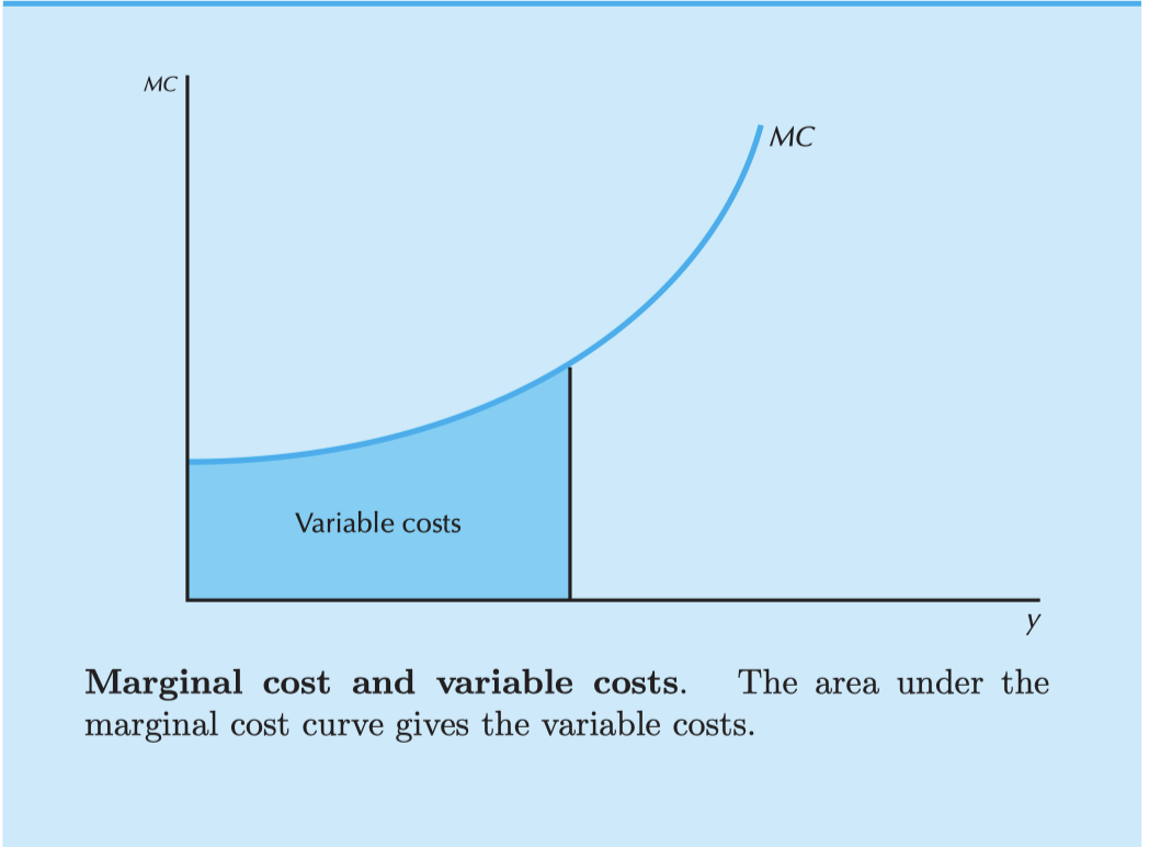
The area under the marginal cost curve measures the variable costs.
The change in producer’s surplus when the market price changes from p1 to p2 is the area to the left of the marginal cost curve between p1 and p2. It also measures the firm’s change in profits.
The long-run supply curve of a firm is that portion of its long-run marginal cost curve that is upward sloping and that lies above its long-run average cost curve.
Even if a firm is making negative profits, it will still be better for it to stay in business in the short run if the price and output combination lie above the average variable cost curve. For in this case, it will make less of a loss by remaining in business than by producing a zero level of output.
We let \(p^∗ = c(y^∗)/y^∗\) be the minimum value of average cost. This cost is significant because it is the lowest price that could be charged in the market and still allow firms to break even.
In the short run, with a fixed number of firms, the supply curve of the industry is upward sloping, while in the long run, with a variable number of firms, the supply curve is flat at price equals minimum average cost.
in an industry with free entry, a tax will initially raise the price to the consumers by less than the amount of the tax, since some of the incidence of the tax will fall on the producers. But in the long run the tax will induce firms to exit from the industry, thereby reducing supply, so that consumers will eventually end up paying the entire burden of the tax.
Economic rent is defined as those payments to a factor of production that are in excess of the minimum payment necessary to have that factor supplied.
The short-run supply curve of an industry is just the horizontal sum of the supply curves of the individual firms in that industry.
The long-run supply curve of an industry must take into account the exit and entry of firms in the industry.
If there is free entry and exit, then the long-run equilibrium will involve the maximum number of firms consistent with nonnegative profits. This means that the long-run supply curve will be essentially horizontal at a price equal to the minimum average cost.
If there are forces preventing the entry of firms into a profitable industry, the factors that prevent entry will earn economic rents. The rent earned is determined by the price of the output of the industry.
The size of the inefficiency can be measured by the deadweight loss—the net loss of consumers’ and the producer’s surplus.
First-degree price discrimination means that the monopolist sells different units of output for different prices and these prices may differ from person to person. This is sometimes known as the case of perfect price discrimination.
Second-degree price discrimination means that the monopolist sells different units of output for different prices, but every individual who buys the same amount of the good pays the same price. Thus prices differ across the units of the good, but not across people. The most common example of this is bulk discounts.
Third-degree price discrimination occurs when the monopolist sells output to different people for different prices, but every unit of output sold to a given person sells for the same price. This is the most common form of price discrimination, and examples include senior citizens’ discounts, student discounts, and so on.
If a firm can charge different prices in two different markets, it will tend to charge the lower price in the market with the more elastic demand.
An oligopoly is characterized by a market with a few firms that recognize their strategic interdependence. There are several possible ways for oligopolies to behave depending on the exact nature of their interaction.
A Nash equilibrium is a set of choices for which each player’s choice is optimal, given the choices of the other players.
Given any set of complete, reflexive, and transitive individual preferences, the social decision mechanism should result in social preferences that satisfy the same properties.
Arrow’s Impossibility Theorem. If a social decision mechanism satisfies properties 1, 2, and 3, then it must be a dictatorship: all social rankings are the rankings of one individual.
- Given any set of complete, reflexive, and transitive individual preferences, the social decision mechanism should result in social preferences that satisfy the same properties.
- If everybody prefers alternative x to alternative y, then the social preferences should rank x ahead of y.
- The preferences between x and y should depend only on how people rank x versus y, and not on how they rank other alternatives.
- Arrow’s Impossibility Theorem shows that there is no ideal way to aggregate individual preferences into social preferences.
The First Theorem of Welfare Economics states that a competitive equilibrium is Pareto effcient.
The Second Theorem of Welfare Economics states that as long as preferences are convex, then every Pareto effcient allocation can be supported as a competitive equilibrium.
Walras’ law states that the value of aggregate excess demand is zero for all prices.
General equilibrium refers to the study of how the economy can adjust to have demand equal supply in all markets at the same time.