

READING 12: TOPICS IN DEMAND AND SUPPLY ANALYSIS
12.1 Elasticity
12.a: Calculate and interpret price, income, and cross-price elasticities of demand and describe factors that affect each measure
Own-Price Elasticity of Demand
Own-price elasticity is a measure of the responsiveness of the quantity demanded to a change in price [negative downward-sloping]
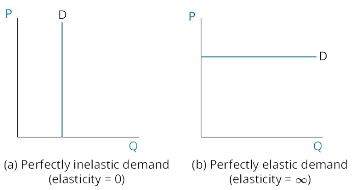
Two Extreme Cases
Factors
- Quality
- Availability of substitutes
- Portion of income spent on a good
- Time
Notice: Elasticity is not equal to the slope of a demand curve
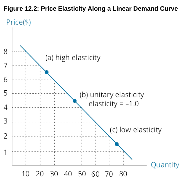
An important point to consider about the price and quantity combination for which price elasticity equals – 1.0 (unit or unitary elasticity) is that total revenue (price × quantity) is maximized at that price.
Income Elasticity of Demand
The sensitivity of quantity demanded to a change in income is termed income elasticity
- normal goods
- inferior good
Cross-Price Elasticity of Demand
The ratio of the percentage change in the quantity demanded of a good to the percentage change in the price of a related good is termed the cross-price elasticity of demand.
- complements
- substitutes
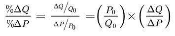
Calculating Elasticities
12.2: DEMAND AND SUPPLY
12.b: Compare substitution and income effects
- The substitution effect is positive, and the income effect is also positive—consumption of Good X will increase.
- The substitution effect is positive, and the income effect is negative but smaller than the substitution effect—consumption of Good X will increase.
- The substitution effect is positive, and the income effect is negative and larger than the substitution effect—consumption of Good X will decrease.
12.c: Distinguish between normal goods and inferior goods
| normal good | inferior good | |
|---|---|---|
| income effect | positive | positive |
A Giffen good is an inferior good for which the negative income effect outweighs the positive substitution effect when price falls. [upward-sloping demand curve]
A Veblen good is one for which a higher price makes the good more desirable. [eg: Gucci bag]
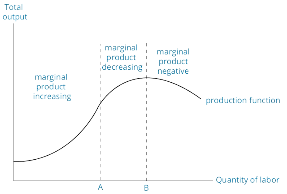
12.d: Describe the phenomenon of diminishing marginal returns
Factors of production are the resources a firm uses to generate output. Factors of production include:
- Land—where the business facilities are located.
- Labor—includes all workers from unskilled laborers to top management.
- Capital—sometimes called physical capital or plant and equipment to distinguish it from financial capital. Refers to manufacturing facilities, equipment, and machinery.
- Materials—refers to inputs into the productive process, including raw materials, such as iron ore or water, or manufactured inputs, such as wire or microprocessors.
12.d: Describe the phenomenon of diminishing marginal returns
12.e: Determine and interpret breakeven and shutdown points of production
In economics, we define the short run for a firm as the time period over which some factors of production are fixed. All factors of production (costs) are variable in the long run.
Shutdown and Breakeven Under Perfect Competition
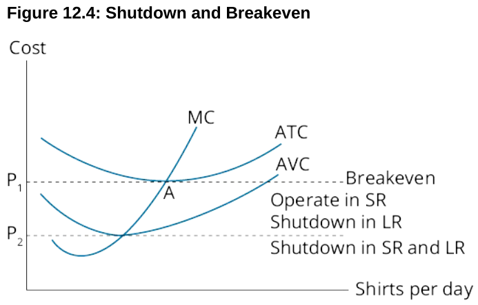
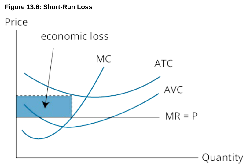
To sum up, if average revenue is less than average variable cost in the short run, the firm should shut down. This is its short-run shutdown point. If average revenue is greater than average variable cost in the short run, the firm should continue to operate, even if it has losses. In the long run, the firm should shut down if average revenue is less than average total cost. This is the long-run shutdown point. If average revenue is just equal to average total cost, total revenue is just equal to total (economic) cost, and this is the firm’s breakeven point.
- If AR ≥ ATC, the firm should stay in the market in both the short and long run.
- If AR ≥ AVC, but AR < ATC, the firm should stay in the market in the short run but will exit the market in the long run.
- If AR < AVC, the firm should shut down in the short run and exit the market in the long run.
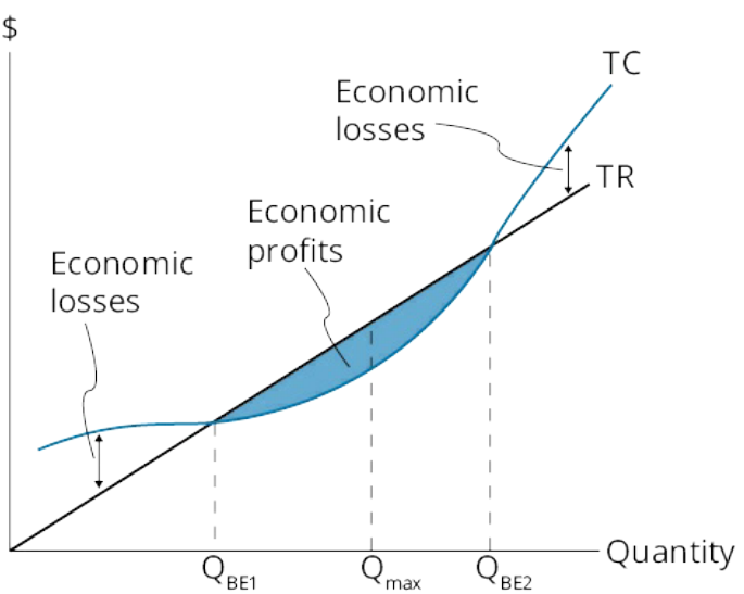
Shutdown and Breakeven Under Imperfect Competition
- TR = TC: break even.
- TC > TR > TVC: firm should continue to operate in the short run but shut down in the long run.
- TR < TVC: firm should shut down in the short run and the long run.
Notice: Marginal revenue is no longer equal to price.
12.f: Describe how economies of scale and diseconomies of scale affect costs
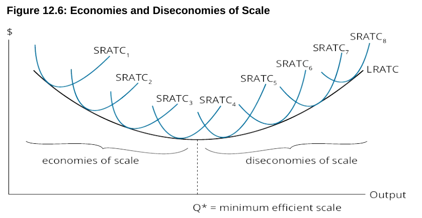
Average total costs first decrease with larger scale and eventually increase. The lowest point on the LRATC corresponds to the scale or plant size at which the average total cost of production is at a minimum. This scale is sometimes called the minimum efficient scale.
Reading 13: THE FIRM AND MARKET STRUCTURES
13.1: PERFECT COMPETITION
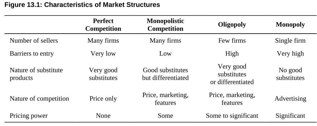
13.a Describe characteristics of perfect competition, monopolistic competition, oligopoly, and pure monopoly.
- Number of firms and their relative sizes.
- Degree to which firms differentiate their products.
- Bargaining power of firms with respect to pricing.
- Barriers to entry into or exit from the industry.
- Degree to which firms compete on factors other than price.
Perfect competition refers to a market in which many firms produce identical products, barriers to entry into the market are very low, and firms compete for sales only on the basis of price.
13.e: Explain factors affecting long-run equilibrium under each market structure.
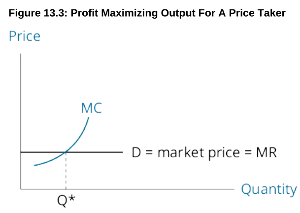
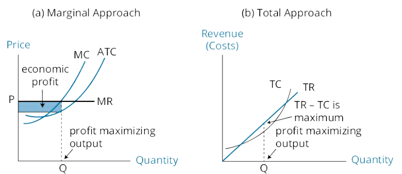
All firms maximize (economic) profit by producing and selling the quantity for which marginal revenue equals marginal cost.
An economic loss occurs on any units for which marginal revenue is less than marginal cost. At any output above the quantity where MR = MC, the firm will be generating losses on its marginal production and will maximize profits by reducing output to where MR = MC.
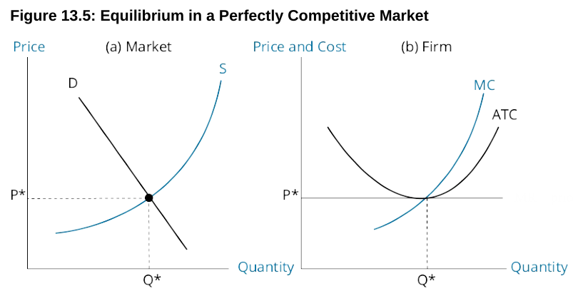
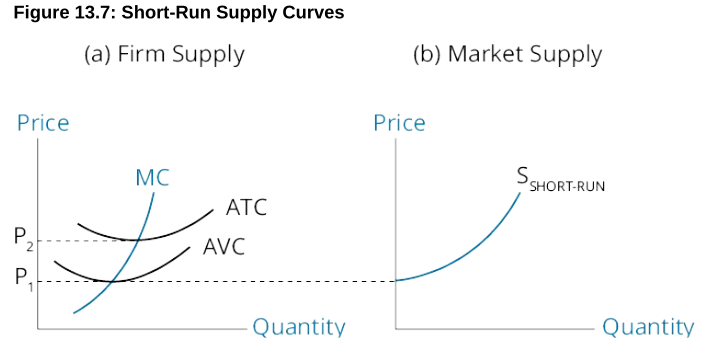
a firm will shut down at a price below P1. Between P1 and P2, a firm will continue to operate in the short run. At P2, the firm is earning a normal profit—economic profit equals zero. At prices above P2, a firm is making economic profits and will expand its production along the MC line. Thus, the short-run supply curve for a firm is its MC line above the average variable cost curve, AVC. The supply curve shown in Panel (b) is the short-run market supply curve, which is the horizontal sum (add up the quantities from all firms at each price) of the MC curves for all firms in a given industry. Because firms will supply more units at higher prices, the short-run market supply curve slopes upward to the right.
Changes in Demand, Entry and Exit, and Changes in Plant Size
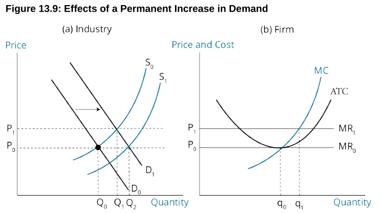
suppose industry demand permanently increases such that the industry demand curve in Panel (a) shifts to D1. The new market price will be P1 and industry output will increase to Q1. At the new price P1, existing firms will produce q1 and realize an economic profit because P1 > ATC. Positive economic profits will cause new firms to enter the market.
13.2: MONOPOLISTIC COMPETITION
market characteristics:
- A large number of independent sellers
- Differentiated products
- Firms compete on price, quality, and marketing
- Low barriers to entry
downwarding-sloping demand curves; highly elastic; competing products are close substitutes
eg: All toothpaste is quite similar, but differentiation occurs due to taste preferences, influential advertising, and the reputation of the seller.
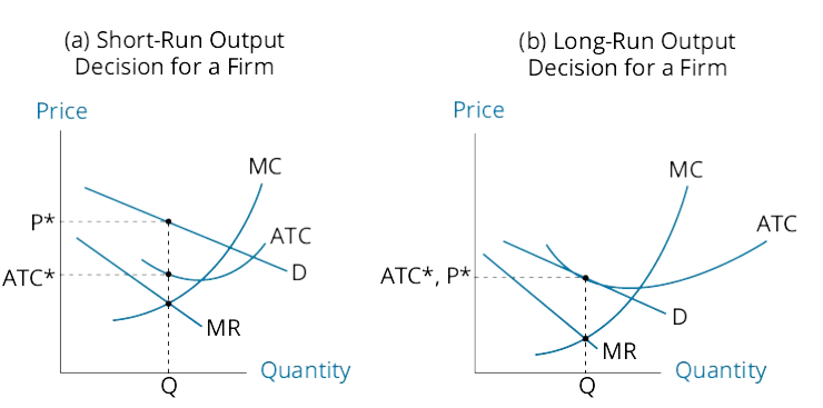
As indicated, firms in monopolistic competition maximize economic profits by producing where marginal revenue (MR) equals marginal cost (MC), and by charging the price for that quantity from the demand curve, D. Here the firm earns positive economic profits because price, P*, exceeds average total cost, ATC*. Due to low barriers to entry, competitors will enter the market in pursuit of these economic profits.
Panel (b) of Figure 13.10 illustrates long-run equilibrium for a representative firm after new firms have entered the market. As indicated, the entry of new firms shifts the demand curve faced by each individual firm down to the point where price equals average total cost (P* =ATC*), such that economic profit is zero. At this point, there is no longer an incentive for new firms to enter the market, and long-run equilibrium is established. The firm in monopolistic competition continues to produce at the quantity where MR = MC but no longer earns positive economic profits.
- Product innovation
- Advertising expenses
- Brand names